Imaging & Photometry
The lecture slides are available here
Make sure you have gone through the setup walkthrough before attempting this! Any issues see Simo (OCW103).
Basic Introduction
Due to strong sky backgound and instrumental noises/effects, we often need to take a few steps to remove these unwanted signals in the raw data to generate images that are suitable for doing science. While nowadays most telescopes have their own automated pinpelines to reduce raw images, it is still very useful to know the basic concepts that goes into these pipelines and to be able to 'debug' if something goes wrong. In this workshop, the goal is to get you to learn these concepts by doing reduction on some real raw data. You will also learn a few useful tools such as SExtractor along the way just so we can generate some prelim science products. While we will use IRAF to demonstrate the steps to reduce raw images, you will also be asked to use your favorite programming language to make some plots.
The Data
By now you should have already downloaded and unpacked the data from:
www.astro.dur.ac.uk/~simo/pg_dr_data/pg_dr_phot.tar.gz
This consists two datasets; in 0220/optical/ you will find the B-band optical imaging data taken by GMOS of cluster RXJC0220.9-3839, and the pre-reduced J/K-band images of the same field can be found in 0220/NIR/. There is also near-infrared imaging data in NIR/ directory of a gravitational lensed galaxy in Cl2243 taken by the NIRC camera on Keck. We use the B-band data on RXJC0220.9 for demonstration. The pre-reduced J/K-band images are for you to do photometric measurements and make scientific plots. Finally the NIR data in Cl2243 are meant for you to practice the reduction processes. Below we give step-by-step instructions for reducing the B-band data.
Reduction Steps
We are now going to reduce the B-band data on RXJC0220.9. Again these are in the 0220/optical/ directory.
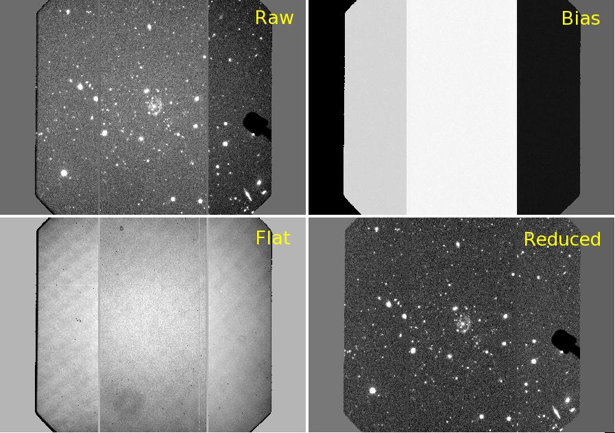
- This directory includes a flat file, a bias file and a set of raw science images. The first step is to subtract the bias off all of the raw science images using imarith in IRAF.
-
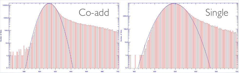
Divide all of the bias-subtracted science images by the flat field using imarith in IRAF. Below shows an example of what these images look like
-
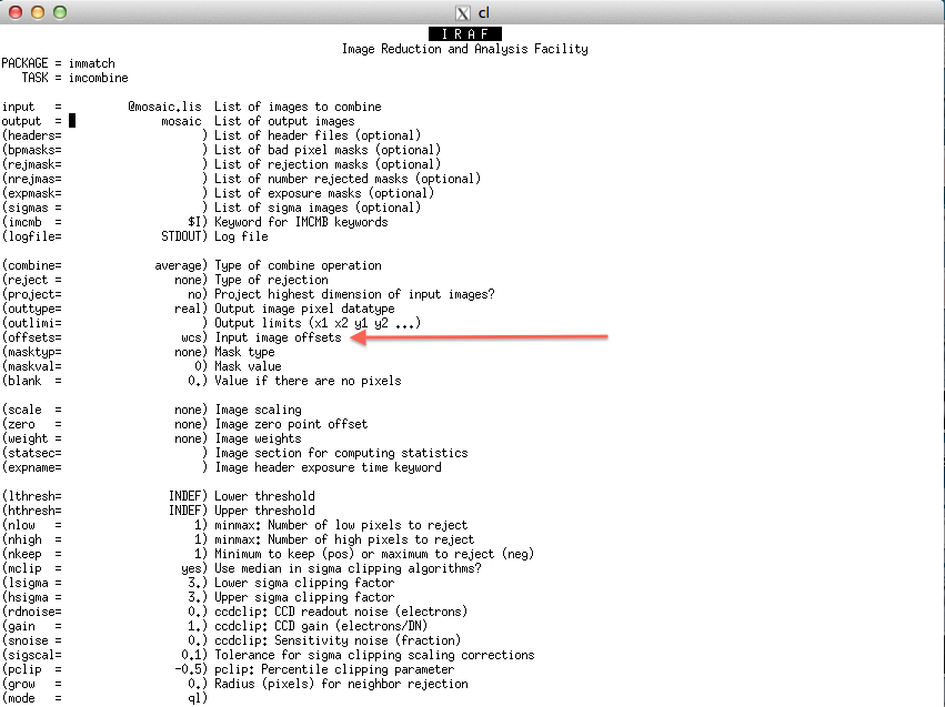
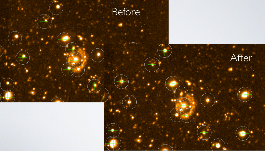
Using imcombine to mosaic the reduced images into a single frame. Don't forget to set the offsets = wcs.
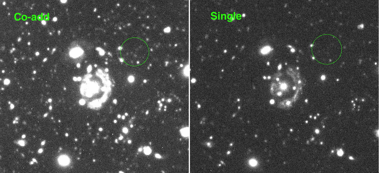
A comparison between the mosaic and single frame images should look like this
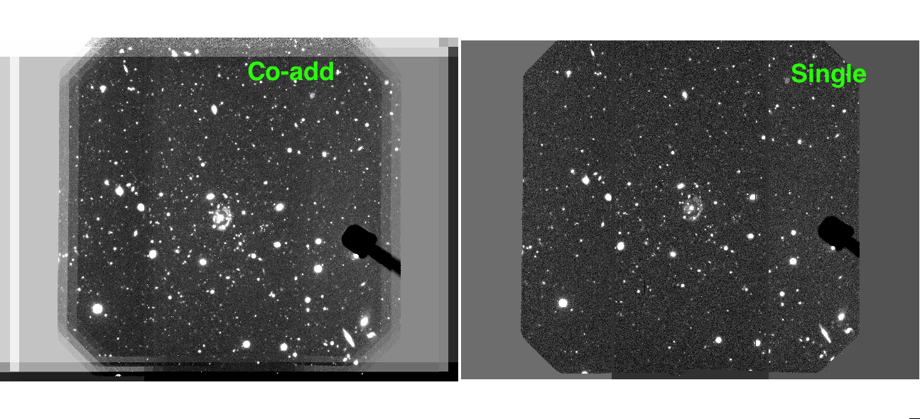
and co-adding makes deeper images
-
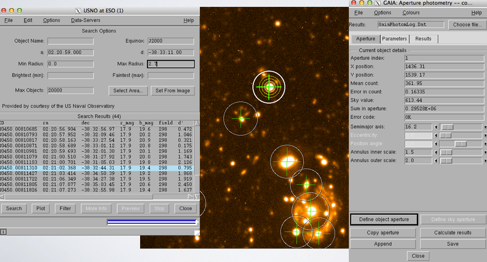
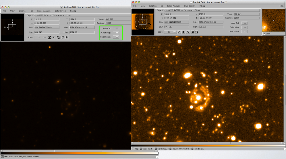
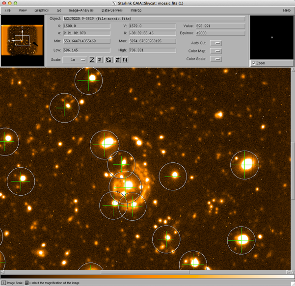
Now we are going to calibrate the astrometry of the mosaic image against know catalog, and we are going to do this in Gaia. First open the mosaic image with Gaia, stretch the image using your favorite color and scale.
Go to Data-Servers -> Catalogs -> bright object catalog USNO at ESO, and then do search.
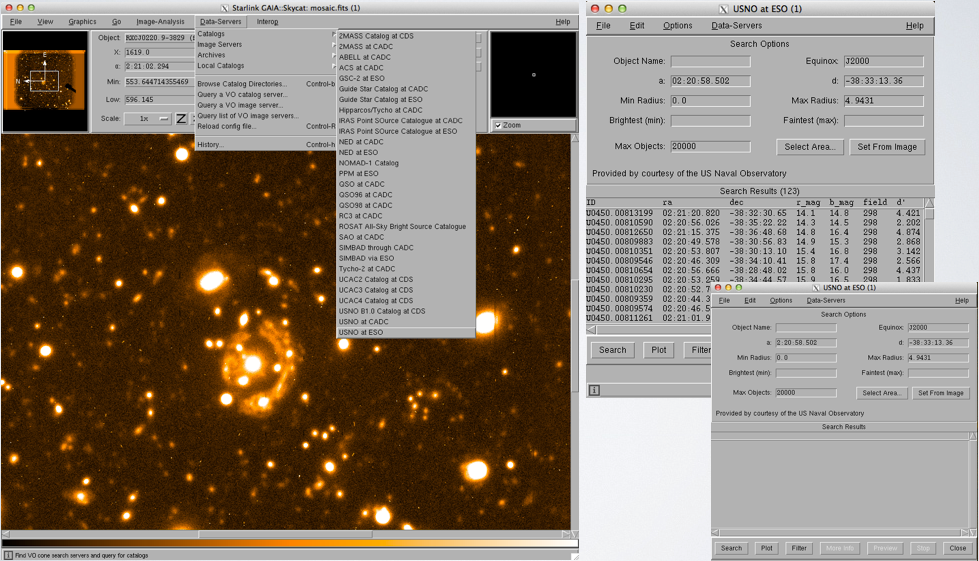
Once you have clicked search, objects should appear, and mismatched positions can be seen.
Next, Image-Analysis -> Astrometry calibration -> Fit to star positions -> Select the USNO at ESO catalog by clicking on "Grab".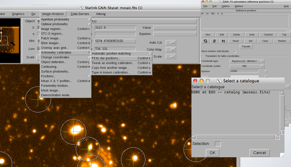
Adjust the marker size and width
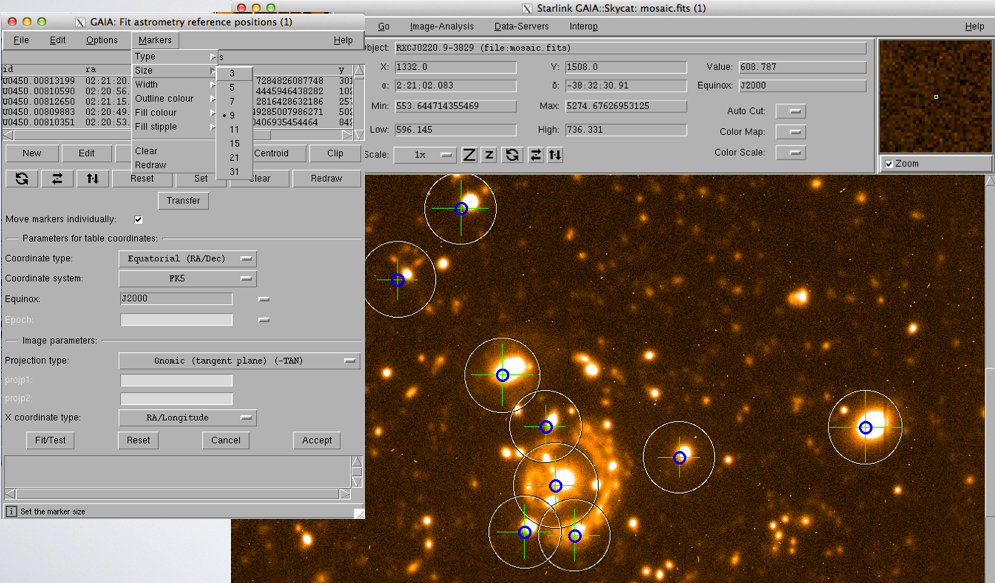
Delete objects outside the frame, delete extended objects and saturated stars.
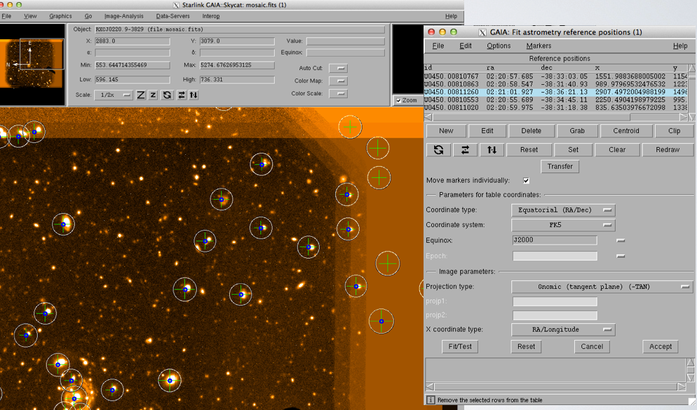
Move markers to the right positions of the bright objects. (Hint: Unclick 'Move markers individually' to move all markers)
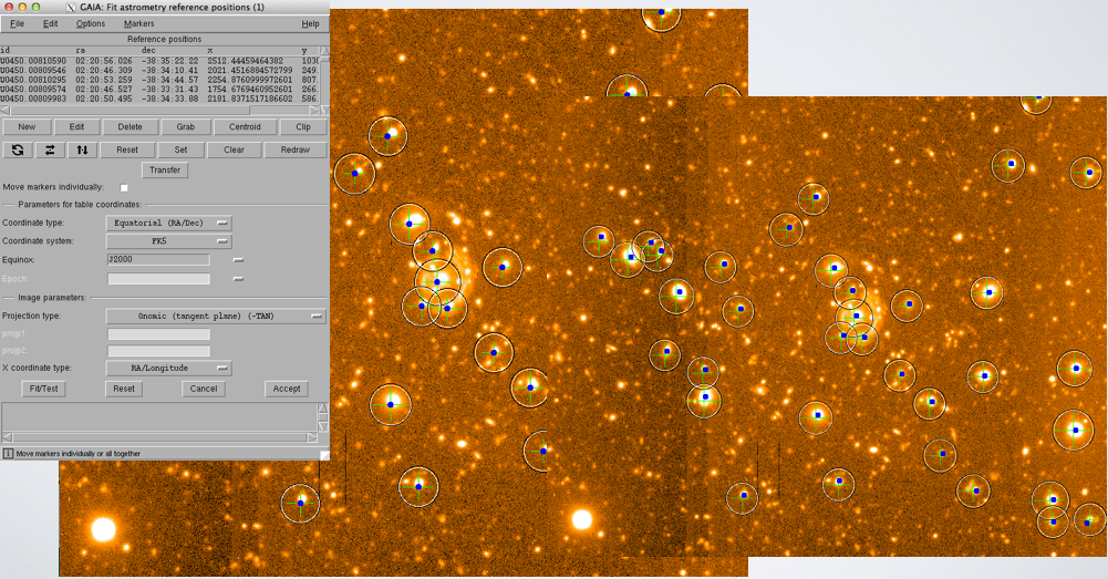
Once all the markers are in the right positions, click Centroid, and then do Fit/Test. Re-center and re-clip and re-fit until the rms reaches less than 0.4'', which is the acceptable values in this data.
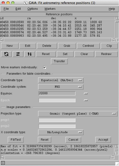
When the fit is good, click Accept and save the image.
-
Very good, we are almost done. The last step is to do flux calibration, as most images have arbitrary digital values, and we need physically meaningful values such as magnitude to do science. The calibration method shown here is to find bright objects with known fluxes, using aperture photometry to measure their flux in arbitrary digital unit, and find the conversion between the digital unit and magnitude.
First, go to Image Analysis in Gaia, and click on Aperture Photometry, and then go to Results in data counts.
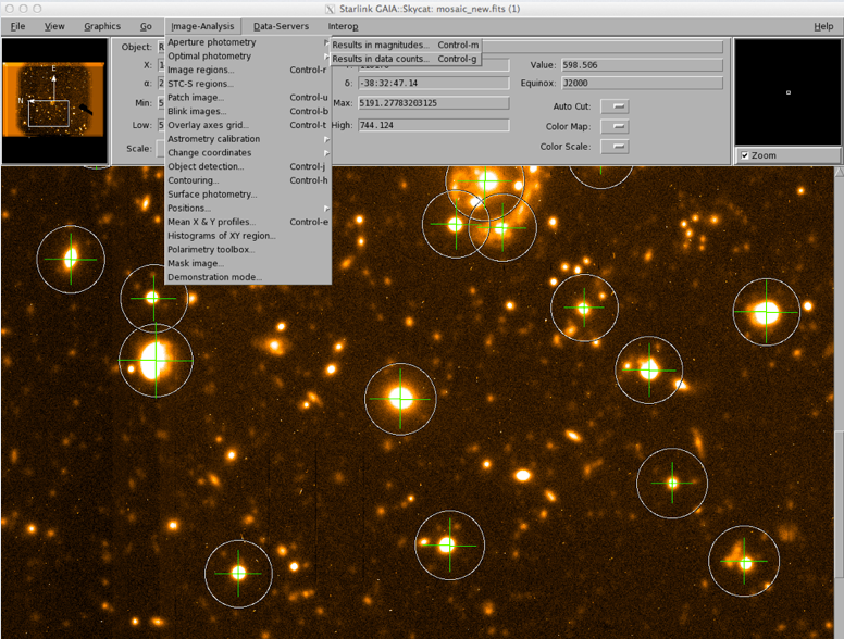
Define an aperture by dragging the cursor -> Calculate results. Finally using the B-band magnitude given in the catalog to calculate the zero point
magnitude = Zpt - 2.5*log(flux)
The zero point is used to convert any flux you measure in the digital unit to magnitude. It is also a critical input parameter for SExtractor, the program to convert the measured flux values to magnitude.
You now have everything that you need to make fully reduced and flux calibrated science images. Well done!
You should now think about some questions and try to answer these during the workshop if time allows. For some of these questions you will need to make use of other tools such as SExtractor, and your favorite programming language for making plots. You are recommended to start working on the questions early and do research to find out how to do some of these tasks (and ask around!).There are also reduced J/K-band images available in 0220/NIR/ directory
(Hint: use hastrom in IDL to align the images (if you can get hold of IDL!). Or your favourite python/other scripting language package)
(Hint: see the SExtractor manual for dual-mode extraction)
Ready for the next task?
If so, head over to the spectroscopy tutorial .