Cathedral view

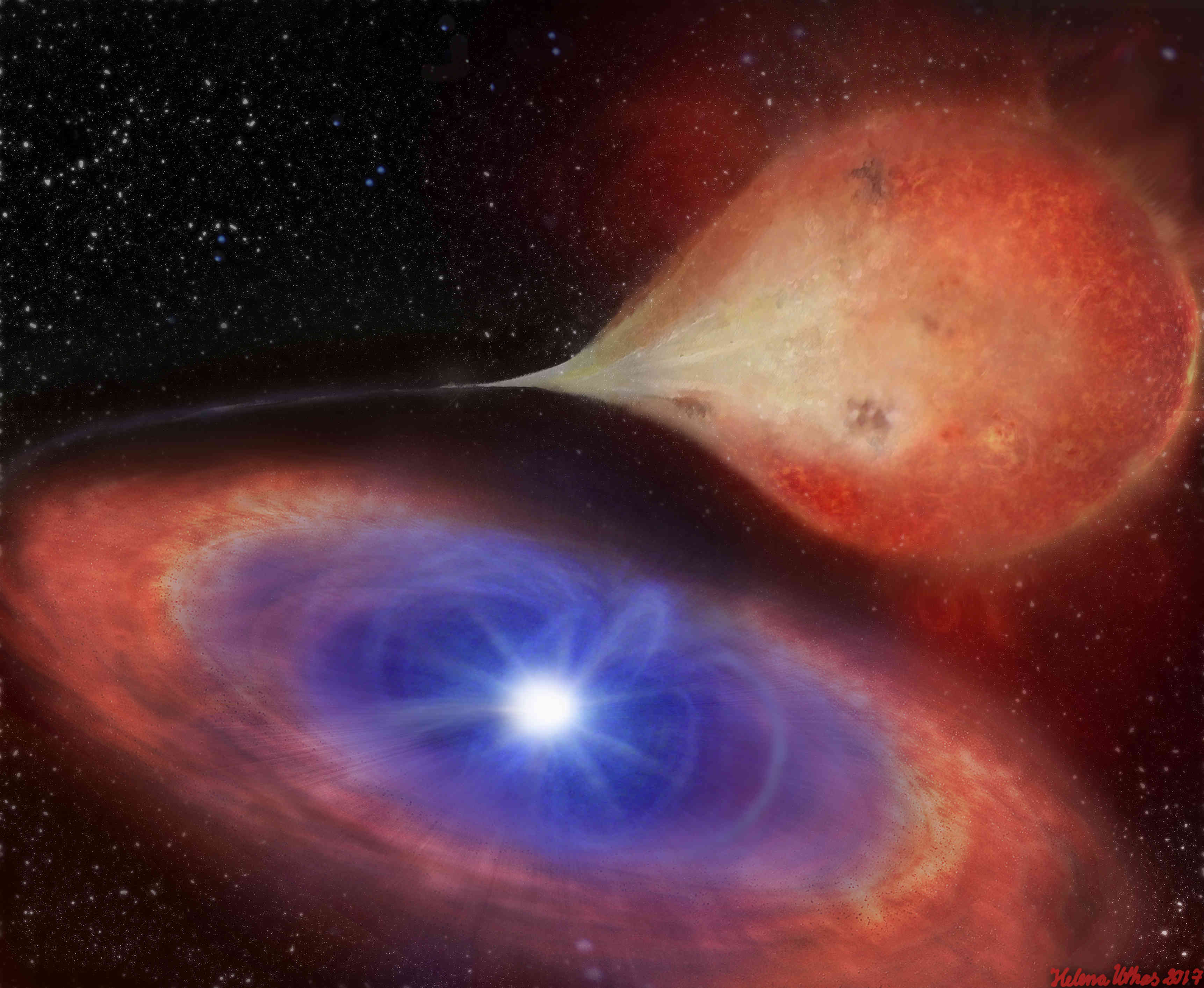
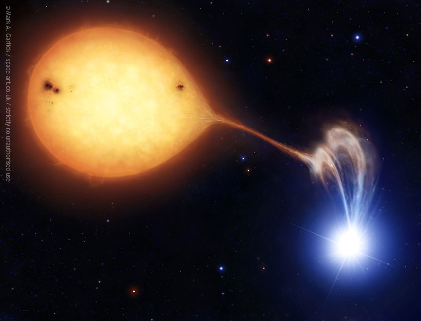
Most stars in the Universe are not alone: they form and evolve in pairs, and in some cases triples or higher hierarchical configurations. In the case of binary systems, the evolution of one of the stars can be faster than its companion. The end result is that the most massive star will evolve into a compact object (either a white dwarf, neutron star, or stellar-mass black hole), while the lower-mass companion wil still be on the so-called main sequence (i.e. still fusing Hydrogen in the core). In this project you will identify known or candidate binaries where a white dwarf is accreting material from the lower mass companion. These systems are usually bright at optical wavelengths, and you will analyse lightcurves (brightness measurments as a function of time) taken from the Physics Department telescopes. You will use these datasets to search for and characterise periodic signals. These signals will reveal the orbital period of the binary systems, and in some cases a secondary signal might also be observed related to the spin period of the accreting white dwarfs.
The goal of this project is to measure and characterise the variability properties of cataclysmic variables. You will do this by producing lightcurves of selected targets and analyse these using Fourier techniques. Here are some suggestions for the project and measurements that you may wish to think about. Note that all data reduction and analysis can either be done in Python or AstroImageJ.
Identify a suitable target (or targets) and the conduct observations. The binary systems you have identified must be known or candidate cataclysmic variables. You can have a look at the known systems in the Ritter & Kolb catalogue, or search for candidate systems thought to have strong magnetic white dwarfs that may reveal a spin period. You can look through the literature, and a suggestion may be to observe X-ray detected cataclysmic variables. See Masetti et al. 2006, and all related papers in that ADS link. Make sure your targets are bright and observable from Durham. Use the exposure time calculator and staralt for this. Choose a filter and exposrure time and conduct observations. Make sure you do not change filters and exposure times throughout.
Calibrate the photometry and astrometry of the individual images. Useful information for this can be found here and here.
Perform relative aperture photometry on each image to generate a lightcurve. You will need to identify your target, as well as a few bright reference stars in the field. To do this you could use AstroImageJ, or use other astronomy software. The end result should be a texty file with 3 columns being: time, flux (or magnitude) and error on flux (or error on magniutude).
Plot the generated lightcurve of your target, as well as some of the reference targets. This should allow you to visually determine if any variability in your target is intrinsic to the target itself, and not a systematic feature also obsewrved in reference stars.
Search for periodicities in the target lightcurve. Do do this you will need to compute a Lomb-Scargle periodogram. This is similar to the Fourier Transform (which you must have heard of previolsy in Electronics or other classes, if not ask), but can handle unevenly spaced data. Once you have a periodogram look at it. Do you see any clear peaks at specific frequencies? If so, what do you think these are?
Compare your periodogram and characteristic frequencies with what is known about the target in the literature. Are your results consistent with what is already known?
Cathedral view
Roof Front-Centre
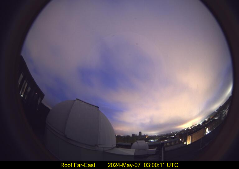
Roof Far-East
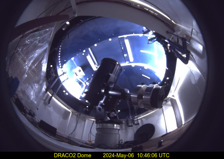
Draco2
East-16
FE20
West-14